Custom ODE (without additional input arguments) Data Generation
The insidapy package can also be used together with custom ODE files to quickly generate different datasets. The following example shows how to use the custom_ode class to generate data from such an ODE file.
This particular notebook explains how to use the codes in case the separete ODE file has NO additional input arguments (i.e., it is a function of the form func(t,x)). In case there are additional arguments, check out the notebook main_custom_ode_with_arguments.ipynb.
First, the custom_ode class is loaded:
[16]:
from insidapy.simulate.ode import custom_ode
Then, the user can define where the separate file with the ODE system is located. The relative path and the filename of the separate function file need to be given as a string. Additionally, the name of the function in the given function file needs to be indicated:
[17]:
CUSTOM_ODE_RELATIVE_PATH = '.'
CUSTOM_ODE_FILENAME = 'customodefile_without_args'
CUSTIM_ODE_FUNC_NAME = 'customode'
Additionally, the user can either add additional parameters that should be passed to the function file by using the ode_arguments input or not. The following example shows the case where no additional parameters are passed to the ODE file. The separate ODE file is located in docs/notebooks/customodefile_without_args:
[18]:
# Give information about the ODE system
CUSTOM_ODE_SPECIES = ['A', 'B', 'C']
CUSTOM_ODE_TSPAN = [0, 3]
CUSTOM_ODE_BOUNDS_INITIAL_CONDITIONS = [[2, 0, 0], [3, 1, 0]]

# Define the units of the ODE system
CUSTOM_ODE_NAME_OF_TIME_UNIT = 'hours'
CUSTOM_ODE_NAME_OF_SPECIES_UNITS = ['g/L', 'g/L', 'g/L']
The separate ODE file could look for example like this (given in markdown format, for the file, check it at docs/notebooks/customodefile_without_args.py):
import numpy as np
def customode(t, y):
        """Custom ODE system. A batch reactor is modeled with two species. The following system
        is implemented: A <-[k1],[k2]-> B -[k3]-> C

        No arguments are used in this function.

        Args:
            y (array): Concentration of species of shape [n,].
            t (scalar): time.

        Returns:
            array: dydt - Derivative of the species of shape [n,].
        """

        # Variables
        A = y[0]
        B = y[1]
        C = y[2]

        # Parameters
        k1 = 4
        k2 = 2
        k3 = 6

        # Rate expressions
        dAdt = k2*B - k1*A
        dBdt = k1*A - k2*B - k3*B
        dCdt = k3*B

        # Vectorization
        dydt = np.array((dAdt, dBdt, dCdt))

        # Return
        return dydt.reshape(-1,)
Similar to the batch-class example above, the instance is created (in case no additional arguments should be passed to the separate ODE function, just ommit the parameter ode_arguments and create the separate function file only by def ODE(t,y)):
Let us use generate only one batch here. We will receive a warning that the number of batches is too little for an LHS sampling method. Automatically, the mid-point of the given upper- and lower bounds is taken as initial condition.
[19]:
data = custom_ode(  filename_custom_ode=CUSTOM_ODE_FILENAME,                        # REQUIRED: Filename of the file containing the ODE system.
                    relative_path_custom_ode=CUSTOM_ODE_RELATIVE_PATH,              # REQUIRED: Relative path to the file containing the ODE system.
                    custom_ode_function_name=CUSTIM_ODE_FUNC_NAME,                  # REQUIRED: Name of the ODE function in the file.
                    species=CUSTOM_ODE_SPECIES,                                     # REQUIRED: List of species.
                    bounds_initial_conditions=CUSTOM_ODE_BOUNDS_INITIAL_CONDITIONS, # REQUIRED: Bounds for initial conditions.
                    time_span=CUSTOM_ODE_TSPAN,                                     # REQUIRED: Time span for integration.
                    name_of_time_unit=CUSTOM_ODE_NAME_OF_TIME_UNIT,                 # OPTIONAL: Name of time unit. Defaults to "h".
                    name_of_species_units=CUSTOM_ODE_NAME_OF_SPECIES_UNITS,         # OPTIONAL: Name of species unit. Defaults to "g/L".
                    nbatches=1,                                                     # OPTIONAL: Number of batches. Defaults to 1.
                    npoints_per_batch=50,                                           # OPTIONAL: Number of points per batch and per species. Defaults to 50.
                    noise_mode='percentage',                                        # OPTIONAL: Noise mode. Defaults to "percentage".
                    noise_percentage=2.5,                                           # OPTIONAL: Noise percentage (in case mode is "percentage"). Defaults to 5%.
                    random_seed=0,                                                  # OPTIONAL: Random seed for reproducibility. Defaults to 0.
                    initial_condition_generation_method='LHS',                      # OPTIONAL: Method for generating initial conditions. Defaults to "LHS".
                    name_of_time_vector='time')                                     # OPTIONAL: Name of time vector. Defaults to "time".
[!] IMPORTANT: It seems that you changed the default bounds of the species. Make sure the order of the indicated bounds is the following: ['A', 'B', 'C']
[!] Warning: You are generating only one batch. Taking the middle point of upper and lower bounds.
After this preparation work, we can run the experiments to create some in-silico data using the run_experiments method. We can then for example check the data of the first experiment.
[20]:
data.run_experiments()
[+] Experiments done.
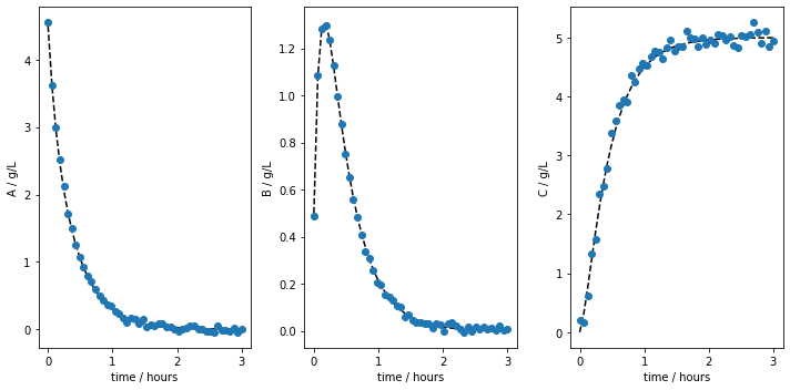
As in the batch class, the generated data can be plotted:
[21]:
data.plot_experiments(  show=True,
                        save=True,
                        figname='custom_odes_with_args',
                        save_figure_directory=r'.\figures',
                        save_figure_exensions=['png'])
[+] Saving figure:
        ->png: .\figures\custom_odes_with_args.png
Most modeling approaches require a training dataset and a separate testing dataset. To generate separate datasets, the user can apply a splitting in an sklearn-manner. There is no default value set. In case the user calls the function, a test_splitratio in the range [0,1) needs to be chosen. The value represents the fraction of the total number of batches generated used for the test set. The data is then splitted and stored in the data object as data.training and data.testing.
[22]:
data.train_test_split(test_splitratio=0.2)
[!] Warning: The number of training batches is 0. All batches are used for testing. Using at least one batch for training now!
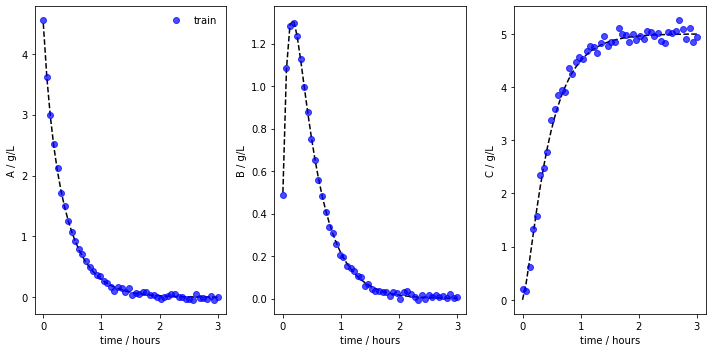
We can now also plot the experiments while showing the training and testing runs individually. The method lets us save the figure using a path (save_figure_directory), a name (figname) and an some extensions (save_figure_exensions) as a list. By using show=False, the plot will not be displayed in a running code.
[23]:
data.plot_train_test_experiments(   save=True,
                                    show=False,
                                    figname=f'{data.example}_custom_ode_train_test',
                                    save_figure_directory=r'.\figures',
                                    save_figure_exensions=['png'])
[+] Saving figure:
        ->png: .\figures\custom_custom_ode_train_test.png
After the simulation, one can export the data as XLSX files. By choosing which_dataset to be training (only executable if train_test_split was applied), testing (only executable if train_test_split was applied), or all (always executable), the corresponding data is exported to the indicated location:
[24]:
data.export_dict_data_to_excel(destination=r'.\data', which_dataset='all')      # Exports all the data
data.export_dict_data_to_excel(destination=r'.\data', which_dataset='training') # Exports the training data
data.export_dict_data_to_excel(destination=r'.\data', which_dataset='testing')  # Exports the training data
[+] Exported batch data to excel.
        -> Dataset: ALL (options: training, testing, all)
        -> Noise free data to: .\data\custom_all_batchdata.xlsx
        -> Noisy data to: .\data\custom_all_batchdata_noisy.xlsx
[+] Exported batch data to excel.
        -> Dataset: TRAINING (options: training, testing, all)
        -> Noise free data to: .\data\custom_training_batchdata.xlsx
        -> Noisy data to: .\data\custom_training_batchdata_noisy.xlsx
[!] WARNING: Test data is empty! Adjust train_test_split ratio!
[+] Exported batch data to excel.
        -> Dataset: TESTING (options: training, testing, all)
        -> Noise free data to: .\data\custom_testing_batchdata.xlsx
        -> Noisy data to: .\data\custom_testing_batchdata_noisy.xlsx